Answers blowing in the wind

For the past several months, I have been working on a model to describe windflow over varied terrain.  The purpose of this model is to calculate average wind motion on a fine grid throughout the day leading up to a possible tornado event, which will later be used to map heat and moisture differences.  I opted to build this model from scratch because existing windflow models (like the wonderful Global Wind Atlas) focus on regional wind climate, too long-term and broad-scale for my analysis.  Also, building a program yourself provides an intimate understanding of the physics/math behind the colorful plot.  That is, as long as you know where to start.

Wind is a complicated subject, turbulent and unpredictable by nature.  Turbulent flow fields are often simulated using computational fluid dynamics (CFD), most commonly a large eddy simulation (LES, see footnote).  But these approaches are computationally expensive – the calculations I’d like to do would take hours or days on my laptop – so I searched for reasonable ways to average out the turbulence.  Despite decades of field research (other footnote), there’s still no consensus method for wind profiling over diverse terrain.  So I made my best attempt to synthesize data from many studies into parameterizations suitable for the rolling-but-not-rugged terrain of the central U.S.

First, I had to understand how sustained winds and gusts behave over homogeneous terrain.  For flat areas with uniform land surface, the mean winds assume a logarithmic velocity profile, with rough surfaces creating additional disturbance close to the ground.  Deviations in speed and direction from the mean profile have been shown to be roughly approximated by Gaussian distributions.  These assumptions are widely used as the basis for regional weather and climate models because they allow for the calculation of fluxes of momentum, heat, and moisture over wide area averages.  To narrow the analysis to small features, I elected to treat terrain differences as “obstacles,” which have been thoroughly described by aerodynamics studies.  Obstacles have two predominant effects on surface-level flow: blocking and channeling.  Linear wind blocking was evaluated point by point for the Gaussian distribution of wind directions at the given wind direction.  A mass balance was applied to these blocking wind profiles to include the effects of flow channeling.  The result was a map that could identify surface eddies in seconds from inputs of average wind speed and direction, shown below:

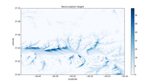
The map represents the SW quadrant of Joplin, MO, and the blue areas identify the persistence of flow eddies in the Shoal Creek valley.  In this plot, the wind was initialized to be 8 m/s from the NW (as in a typical cold front), and the scale bar indicates the height of recirculation eddies in meters.  While preliminary tests have shown that this model compares well to the Global Wind Atlas’s orographic speedup feature, I am curious whether this model’s simplicity would hold up to field experiments or more complex terrain features.  Either way, I am excited to implement the next step on top of this wind model: a detailed heat and moisture map of the boundary layer.

 

Footnote: For practical purposes, research meteorologists most often use a Large Eddy Simulation (LES) to simulate wind flows, which simplifies the Navier-Stokes Equations by lumping small turbulent motions into a ‘dissipation’ term.  This approach will be essential when I want to model the physics of tornado motion, but not critical for boundary layer modeling.

Other Footnote: Potentially game-changing research is happening in this area, which could one day lead to a consensus.  The NSF-funded Perdigao project, begun in Spring 2017, seeks to resolve wind fields over complex hilly-to-mountainous terrain in Portugal. This dataset should be far more comprehensive than the current standard taken in the 1980s around Scotland’s Askervein Hill.

Title Credit: Bob Dylan

#BombCyclone: the latest Nor’easter

We survived Snowmageddon*.  Then a few Snowpocalypses. This time, the Polar Vortex teamed up with the ocean that gave us Superstorm Sandy to produce…a bomb cyclone named Grayson!

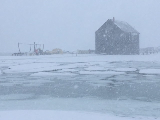
Grayson on Thursday, bearing down on the Northeast like an ice cold hurricane (GOES16-East imagery, source: NASA).

Histrionics aside, I don’t want to downplay the severity of this week’s winter storm. It was historic in its own right, dumping a foot of snow on much of the Eastern Seaboard, flooding coastal areas in New England, and claiming at least 8 lives. Places like Savannah, GA woke up under a blanket of snow for the first time in 30 years. Record low temperatures have followed for much of the east coast, exacerbating the dangers for those without power (especially in the Southeast, where snow is rare and snowplows even rarer). A deep freeze will keep the snow around for several days, and people who don’t live in Maine are forced to get a week-long taste of the Maine winter.

After all, this meteorological setup is normal for Maine. Colloquially called a Nor’easter, winter storms like these can dump upwards of a foot of snow one or more times a year.  They form when a sharp temperature gradient exists between the arctic and subtropical Atlantic air masses. The mixing of these air masses generates a low pressure system wherein the humid ocean air lifts and precipitates as heavy snowfall, and the system becomes a bomb cyclone if the minimum pressure within the system drops more than 24 millibars in 24 hours (i.e., undergoes “bombification”, yes these are real meteorological terms).  While this storm moved through its lifecycle unusually quickly – bombifying near the Carolinas then landfalling in Nova Scotia within 36 hours – this storm had many well-known precedents, most recently winter storm Juno in 2015.

Which is why we need to talk about how storms are named.  The Weather Channel assumed the unofficial duty of naming winter storms beginning in November 2012.  Storms had previously been identified by catchy puns that went viral, as the early days of social media were dominated by Snowtobers and Icepocalypses and Snowmageddon.  The Weather Channel capitalized on the use of hashtag-able names as a way to generate interest and increase views, but the NWS and Accuweather denounced their naming practice. However, this rejection of arbitrary names led to the adoption of obscure meteorology terms as storm identifiers, such as the polar vortex (2013), bomb cyclone (2018), and winter superstorm (2014).  In my opinion, this appropriation of technical vocabulary for clickbait purposes is more dangerous, as it gives the impression that severe winter storms are increasing in frequency and magnitude.  Of course, a single weather event cannot be directly attributed to global climate change, but every hyped-up winter storm provokes articles from climate change alarmists and skeptics alike.  What we really need is a standard language for communicating information about impending winter storms, ideally paired with a ratings system that objectively tracks storm severity.  This system already exists in the Northeast, called the Northeast Snowfall Impact Scale (NESIS), and I think similar scales should be adopted nationwide.

Sea ice at Derby Wharf in Salem, Massachusetts – yes, this photo was in fact taken in 2018. Source: Patch

*The winter storm of February 5-6, 2010 was widely referred to as Snowmageddon, famous at the time for dumping over 2 feet of snow on much of the Mid-Atlantic.  Clearly, it wasn’t the end of the world.